Introduction

In the previous blog post we introduced the problem of sample bias along with an example where it could lead to a subpar classifier being selected. We also discussed how sample bias can affect statistics like the estimated probability of support for a candidate. That post contained several techniques and suggestions for correcting sample bias, and in this post we’re going to take a deeper look at those and see how, under the surface, bias correction all comes from a single thing: rescaling expectations with Radon-Nikodym derivatives.

Motivation

We'll begin by introducing our notation and reviewing the two situations described in the previous post where sample bias can occur. We’ll then show how they’re both special cases of the same general quantity and the correcting factor is fundamentally the same.

Notation: we will be exploring cases where we observe data where is a random covariate vector, is the response, and all samples of random variables are independent and identically distributed. Often we will take to be binary but in general it is unrestricted. We will be considering expectations with respect to various distributions so will be used to denote the expected value of a random variable with respect to a distribution . All of this is in the context of sample bias, so we will let be the joint distribution of in the training set and will be the joint distribution of in the population of interest (also called the test set). and (without asterisks) will denote the marginal covariate distributions, and the corresponding covariate densities will be and respectively. 

First, we will consider supervised learning. In statistical learning theory, a particular model is chosen from the class of models under consideration by minimizing the risk which is the expected loss when using to predict . Because the distribution is unknown this expectation is unavailable, so we instead choose our model to be the minimizer of the empirical risk

which, under certain conditions, converges to . If, however, our data comes from a different distribution than that of the population of interest we will be minimizing the wrong quantity: our empirical risk will converge to rather than so we could select the wrong model. We saw an example of this in the previous post, and how we can correct this by adding weights to the loss function to encourage the model to perform better on the samples that are more likely under

Next, we will consider survey sampling. Frequently we are interested in estimating the population prevalence of something, which is of the form . If our training data is distributed according to then this can be estimated via the sample average

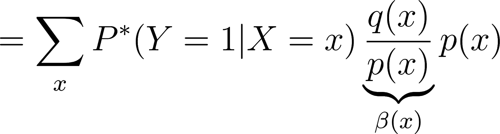
If, as in our current situation, the data instead is distributed according to then will converge to the wrong thing and our estimate is off. In the previous post we discussed multilevel regression and poststratification (MRP) as a way to fix this. This is a technique where we bin the covariates and then estimate via

i.e. we sum estimates of the conditional probabilities (obtained via a multilevel logistic regression) over all possible , weighted by the test set probability of that . Note how for a binary we have .

These two problems look quite different on the surface, but in both cases they come down to needing to estimate a quantity of the form with data drawn from a different distribution . In the first case, we have while in the second (where is the indicator function for the event ). As we shall see, with two key assumptions there exists a function such that

so our bias corrections are completely given by . This function is a Radon-Nikodym derivative (RND).

Radon-Nikodym Derivatives

In order to discuss Radon-Nikodym derivatives we need to fix a collection of events to which we can assign probabilities. Such a collection is called a -algebra. A probability measure is a function from into that does this assigning and behaves in a way consistent with how we expect probabilities to work; for example, the probability of the union of two disjoint events ought to be the sum of the probabilities of each event on their own.

For an example of a -algebra, let's say we perform an experiment where we toss a coin once. Then our -algebra will be because these are all of the events that we can and want to assign probabilities to. We could then define a probability measure on by saying (this is the probability of the event that the coin comes up heads), (this is the probability that the coin comes up heads or tails), (this is the probability of tails), and (this is the probability that the coin doesn’t come up anything which is impossible). Note that because of the rules of probability like (where is the complement of ) we actually in this case only needed to give the value for in order to completely specify the distribution. It makes intuitive sense that the probability that a coin comes up heads is sufficient to completely characterize its distribution. In this example, we have a biased coin that comes up heads 30% of the time.

Returning to our general -algebra , let and be two arbitrary probability measures on it. The Radon-Nikodym theorem asserts that if for every (denoted , and referred to as the assumption of nested supports), then there exists a non-negative function such that

for every event . We denote this by . The reason RNDs are so great is that they allow us to "rescale" a potentially hard to study measure into a much easier one. As an example of turning a difficult integral into a tractable Riemann integral, consider a probability measure given by

and defined on a suitable -algebra over (typically the Borel -algebra). Here will denote the Lebesgue measure which generalizes the standard notion of length (e.g. ), and it turns out that integrals with respect to exactly generalize Riemann integrals, such as here, and in many cases coincide. This justifies our change of notation later from to just .

Note that if then necessarily so the RND exists, and in fact is sitting right in front of us:

In particular, our RND in this case is exactly the probability density function (PDF) of a standard Gaussian random variable. So if we have a random variable with as its distribution then by definition the expected value of is

This isn’t a very useful form for evaluating this integral, though, because we’re integrating with respect to a complicated measure . If instead we could make this a Riemann integral then we’d have something we know how to do, and indeed that’s exactly what we can do with our RND:

so now we’ve got a friendly Riemann integral, and using a change of variables we can see that it’s equal to 0.

As this example hints at, we use RNDs all the time in probability without saying it: every PDF and probability mass function (PMF) is an RND. Keeping as the Lebesgue measure and letting be the counting measure (this gives the cardinality of a set), then a PDF is nothing more than an RND of some probability measure with respect to and a PMF is an RND of some other probability measure with respect to . We saw this above in that the standard Gaussian PDF is exactly an RND of a probability measure with respect to the Lebesgue measure. 

Also it’s worth noting how in the above example with , our measure is a function that takes sets as its inputs so it is naturally quite tricky to visualize. The RND, however, is a function from to so we can quite easily plot it and gain intuition from this. This convenience and intuitive appeal is a big part of why basically all of our nice named distributions (e.g. Gamma, Beta, Gaussian, Cauchy, etc) are specified by their Lebesgue RNDs rather than by their measures.

One thing to note is that, by virtue of being defined inside of an integral, RNDs are defined only up to sets of measure zero: if then we can change ’s values on without affecting the results at all. Typically there is a ‘canonical’ RND but this point is worth remembering (it does turn out to be the case that RNDs are unique aside from changes on sets of measure 0).  

Now that we have a sense of what an RND is, we will need one particular property of them that will come up later: if there exists a probability measure such that then

i.e. the RND is equal to the ratio of RNDs both with respect to a different measure . The advantage to this is that in many practical cases we can produce a with these properties such that and are far easier to work with than the original . For example, if this is true with then we can compute our abstract RND as the ratio of two Lebesgue PDFs which will almost certainly be easier to do.

Returning to sample bias

We have our probability measures and . We first want to find a function with the property that

Recalling the definition of expectation, we have

and we want to turn this into something of the form

By inspection we can see that we need to take

and in order for this to exist we need nested supports, i.e. (recall that this means that if then too). As we mentioned in the previous post, intuitively this assumption says that in order for correction to be possible there can't be any test points that have a probability of 0 of appearing in the training set.  

There is a problem with what we have so far: depends on . Frequently this will prevent us from being able to estimate it. For example, in the previous post our example had to make do with unlabeled covariates drawn from because were unavailable (and indeed, if they were available then we wouldn’t have sample bias). So we will need to make a second assumption, that of covariate shift, to eliminate from our RND.

Covariate shift is the assumption that the distribution of given is the same under both and . This is definitely a non-trivial assumption, but as we've said, it is difficult to get anywhere without it. Once we've made that assumption, it turns out that effectively cancels from and we find that

provides the correcting factor. 

All together, we now have that

Estimating through the Iterative Proportional Fitting Procedure or Kernel Mean Matching 

Recall the property of RNDs that we may sometimes produce a measure such that

This property is exactly the reason that our bias correction can be obtained as the ratio of two PMFs or PDFs, as in the example in the previous post. In that example, both our covariate distributions were multivariate Gaussians so we could take , and indeed that's what we were tacitly doing when we used the ratio of PDFs to get the bias correcting weights.

If instead we are binning our features, this has the effect of making the condition hold for (still assuming ), which means we can compute as the ratio of covariate PMFs. This is exactly what was accomplished by using the Iterative Proportional Fitting Procedure of the previous post.

There are also techniques that avoid computing a ratio of densities, including Kernel Mean Matching (KMM). This technique directly models as an element of a function space and solves a quadratic program to obtain the vector of evaluations of on the training points. This has the advantage of being more efficient in that rather than estimating an entire function we instead only obtain its values in the places we care about. We also avoid high dimensional density estimation.

See here for more: https://papers.nips.cc/paper/3075-correcting-sample-selection-bias-by-unlabeled-data.pdf.

 

Putting RNDs in our examples 

Here we'll go through our two examples and show how to put RNDs in them.

For the supervised learning example, we just need to use a weighted empirical risk 

Once we have our evaluations this is easily done in most modern machine learning toolkits, such as scikit-learn.

For the survey sampling example, we could use a weighted average

as our estimate.

This weighted average does do the trick but it doesn't make the connection to MRP clear. As in MRP, assume all of our predictors are discrete. The Law of Iterated Expectations is a result that says

Applying this to our problem, we have

We know

and under covariate shift

so we have

So in the case of MRP we can write our estimator in the form of a RND-corrected expectation, although the value of this is in seeing the relationship with other techniques rather than computational.

Conclusion 

We have seen that under the assumptions of nested supports and covariate shift there exists a function such that we can correct an expectation of with respect to into an expectation with respect to a different distribution . We have also seen two examples to show that quantities of this form (i.e. ) are quite ubiquitous so this is a useful thing to be able to do, and in particular we have seen how sample-level weights for bias correction in supervised learning and cell-level averaging in MRP are, at a fundamental level, both justified by the same result.

One thing we have so far glossed over is the difference between population and sample results. In all of this, we have made use of population quantities like . If we are estimating these from data, as we will have to do, it is no longer necessarily the case that these results exactly hold. For further discussion on this distinction between population and sample, see "An improved categorization of classifier's sensitivity on sample selection bias" by Fan et al (2005), found here: http://ieeexplore.ieee.org/document/1565737/. There is also the issue of the extra variance incurred, and while the RND may be the correct weighting function in the population sense it may be too high variance to estimate for a finite sample.